Principal Component Analysis
General Principles
Principal Component Analysis (PCA) (Tipping and Bishop 1999) is a technique used to reduce the dimensionality of a dataset by transforming it into a new coordinate system where the greatest variance of the data is projected onto coordinates (called principal components). This method helps capture the underlying structure of high-dimensional data by identifying patterns based on variance.
In Bayesian PCA, uncertainty in the model parameters is explicitly taken into account by using a probabilistic framework. This allows us to not only estimate the principal components but also quantify the uncertainty around them and avoid overfitting by incorporating prior knowledge.
PCA is employed for dimensionality reduction, particularly in scenarios involving high-dimensional datasets, as it effectively reduces complexity while explicitly accounting for uncertainty in the underlying latent structure. This approach also plays a crucial role in data visualization, enabling the projection of intricate, high-dimensional data into more interpretable 2D or 3D representations. Additionally, PCA excels in feature extraction, where the latent variables it identifies can be repurposed as informative features for subsequent tasks, such as classification or clustering. By modeling latent variables, it further enhances the interpretability and utility of the data for a variety of analytical applications.
Considerations
In Bayesian PCA, we assume prior distributions for the latent variables Z and the principal component loadings W. We place Gaussian priors on both Z and W and learn their posterior distributions using the observed data X.
Robustness to Outliers: Standard PCA are sensitive to outliers due to the assumption of Gaussian noise. Robust variants of Robust Bayesian PCA address this by employing heavy-tailed distributions for the noise model, such as the Student’s t-distribution, which reduces the influence of outliers (Archambeau, Delannay, and Verleysen 2006; Bouwmans and Zahzah 2014).
Automatic Dimensionality Selection: Through techniques like Automatic Relevance Determination (ARD), Bayesian PCA can automatically determine the effective dimensionality of the latent space. Priors are placed on the relevance of each principal component, and components that are not supported by the data are effectively “switched off’ (C. Bishop 1998; C. M. Bishop and Nasrabadi 2006).
Sparsity for High-Dimensional Data: In high-dimensional settings, it is often desirable for the principal components to be influenced by only a subset of the original features, leading to more interpretable results. Sparse Bayesian PCA achieves this by placing sparsity-inducing priors (e.g., Laplacian or spike-and-slab priors) on the loading (Sigg and Buhmann 2008; Zou, Hastie, and Tibshirani 2006).
Example
Here is an example code snippet demonstrating Bayesian PCA using BI:
from BI import bi,jnp
m=bi()
data_path = m.load.iris(only_path=True)
m.data(data_path)
m.data_on_model = dict(
    X=jnp.array(m.df.iloc[:,1:4].values)
)
m.fit(m.models.pca(type="classic"), progress_bar=False) # or robust, sparse, classic, sparse_robust_ard
m.models.pca.plot(
    X = m.df.iloc[:,1:4].values,
    y = m.df.iloc[:,5].values,
    feature_names = m.df.columns[1:4],
    target_names = m.df.iloc[:,6].unique(),
    color_var = m.df.iloc[:,1].values
)
def model(x_train, data_dim, latent_dim, num_datapoints):
# Gaussian prior for the principal component 'W'.
w = m.dist.normal(0, 1, shape=(data_dim, latent_dim), name='w')
# Gaussian prior on the latent variables 'Z'
z = m.dist.normal(0, 1, shape=(latent_dim, num_datapoints), name='z')
# Exponential prior on the noise variance 'epsilon'
epsilon = m.dist.exponential(1, name='epsilon')
# Likelihood
m.dist.normal(w @ z , epsilon, obs = x_train)
m.data_on_model = dict(
x_train=x_train_h,
data_dim=data_dim,
latent_dim=4,
num_datapoints=num_datapoints
)
m.fit(model)using BayesianInference
m = importBI(platform="cpu")
data_path = m.load.iris(only_path=true)
m.data(data_path)
m.data_on_model = pydict(
X=jnp.array(m.df.iloc[:,1:4].values)
)
m.fit(m.models.pca(type="classic"))
# ------------------------------------------------------------------------
# ⚠️ Forcing Matplotlib to use the "Inline" backend for jupyter notebook
# ------------------------------------------------------------------------
plt = pyimport("matplotlib.pyplot")
# 1. Create empty contexts
globals_dict = pybuiltins.dict()
locals_dict = pybuiltins.dict()
# 2. Define the dummy function safely
dummy_show = pybuiltins.eval("lambda *args, **kwargs: None", globals_dict, locals_dict)
# 3. Save the real show function
real_show = plt.show
# 4. Overwrite
plt.show = dummy_show
# 5. Run your plot
m.models.pca.plot(
X = m.df.iloc[:,1:4].values,
y = m.df.iloc[:,5].values,
feature_names = m.df.columns[1:4],
target_names = m.df.iloc[:,6].unique(),
color_var = m.df.iloc[:,1].values
)
# 6. Restore real show
plt.show = real_show
# 7. Display the result
display(plt.gcf())
plt.close()Mathematical Details
We assume the observed data matrix X is centered and arranged with features as rows and samples as columns, X \in \mathbb{R}^{N \times V} where N is the number of observations and V the number of variables. The generative model projects the data into a lower-dimensional space with K latent variables, K \leq V, using the following equation: X \sim \text{Normal}(Z \cdot W, \sigma)
where :
X is the observed data matrix.
Z \in \mathbb{R}^{N \times K} is the latent variable matrix (latent features) with K \ll D. Z is defined by a Normal distribution with mean 0 and variance 1.
W \in \mathbb{R}^{K \times V} is the matrix of principal components (projection matrix). W is defined by a Normal distribution with mean 0 and variance 1.
\sigma is the standard deviation of the normal distribution.
The likelihood and priors are defined element-wise for v=1...V, n=1...N, and k=1...K. for the following models:
Standard PCA
X \sim \text{Normal}(Z \cdot W, \sigma) Z \sim \text{Normal}(0, 1) W \sim \text{Normal}(0, 1) \sigma \sim \text{Exponential}(1)
Note
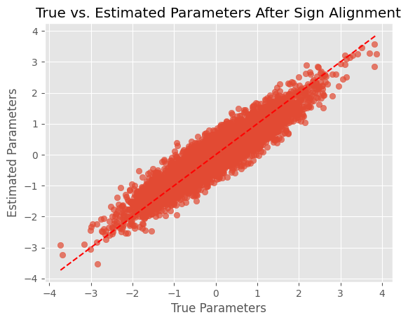
- To account for sign ambiguity 🛈 in PCA, we can set the number of latent dimensions K to be equal to the number of variables V. Then, we can calculate the dot product between the estimated parameters and the data. If it is negative, we multiply the estimated parameters by -1 to align them with the data. Below, a code snippet highlights how to do this:
true_params = jnp.array(real_data)
estimated_params = jnp.array(m.posteriors)

# Compute dot product
dot_product = jnp.dot(true_params, estimated_params)

# Align signs if necessary
if dot_product < 0:
    estimated_params = -estimated_params

# Plot the aligned parameters
plt.scatter(true_params, estimated_params, alpha=0.7)
plt.plot([min(true_params), max(true_params)], [min(true_params), max(true_params)], 'r--')
plt.xlabel('True Parameters')
plt.ylabel('Estimated Parameters')
plt.title('True vs. Estimated Parameters After Sign Alignment')
plt.show()